Chapter 4 Data munging with dplyr
In this chapter you will learn about working with packages, which I find similar to teaching your R new tricks.
I will also introduce you to the tidyverse - a collection of packages and why I strongly suggest to familiarize oneself with a bunch of them.
Spoiler: It will make your life a lot easier.
4.1 Working with packages
First off, when you stick to the metaphor a package being a collection of tricks to teach your R, then you will teach the tricks once and remind R that it knows the tricks every time you want to use them. In more real life terms, you will install a package once and load it in each new session. This is important to remember because installing packages is one of the few things you will only want to do in your console - NOT in any of your scripts. Nothing bad will happen if you do, but it takes a very long time and it will test both your own patience and that of your computer.
Generally, packages can be installed with the install.packages() function.
It needs the package name in quotes as input in the parentheses, e.g. install.packages("dplyr").
This means the package is now on your computer but you still need to make it available.
The easiest way to achieve that is to load the whole package using the library() command.
This will usually be done inside a script where you want to use functions from that package.
Later in this chapter, when we look at dplyr functions on the iris data in Section 4.3, you will see a code chunk as a prototype of a typical beginning of an R script.
While library() makes all functions from a package available, you can also only load specific functions right when you want to use them.
This works with the notation package::function() and is particularly useful if (1) the package is extremely large, takes a long time to load and/or you really only need the one function or (b) the function name you want to use is not unique, i.e. there are several packages that contain a function of that name.
For example, the function filter exists in more than one package, so you might use dplyr::filter() in your code to make explicit that you want to use the filter() function from the dplyr package.
When this is the case, you will get the message "The following objects are masked from..." in the console when you load the package. This is also good to keep in mind if you run into unexpected errors - maybe you meant to use the function from another package but R is using the one you loaded last?
In the interest of creating reproducible code, it can also make sense to use the package::function() notation, so you can explicitly show others which function you used.
At a glance:
- Install packages with
install.packages()only once in the console! - Load packages with
library()every time you load a script or start a new session- Usually in the script, but also in the console
- Specific function from a package:
package::function()- Use if you just need that one function once and don't want load the entire package
- Or to explicitly show the according package
- Or the function name is also in other packages (e.g. "filter" is usually
dplyr::filter, but sometimesstats::filter)
4.2 The tidyverse
The tidyverse is an opinionated collection of R packages designed for data science. All packages share an underlying design philosophy, grammar, and data structures. (tidyverse.org)
So packages are pretty cool: They usually come from people who had a specific problem, found a solution and decided to share it with others so they can more easily fix new problems.
Of course everyone has a different preference on how to work, which is why not every package and function will be intuitive to everyone.
That is also why the definition of an "opinionated collection of R packages" is so fitting because the tidyverse is a framework consisting of many different packages that the authors find intuitive and useful.
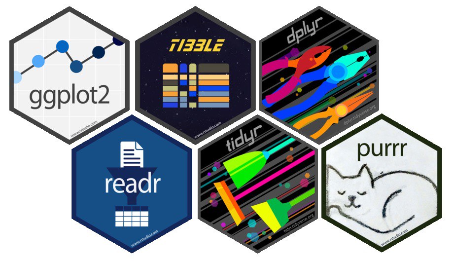
Figure 4.1: Hexagonal package logos of some common R packages.
Incidentally, I agree and I will show you why. If you figure out at some point that your prefer another way - that's great, but the tidyverse is a solid starting point for most data science needs in psychology.
The structure of the tidyverse packages is very clear and they each serve a distinct purpose.
Taking a real-life workflow as inspiration, we will first get to know dplyr, a package for cleaning up data and editing everything to your needs in this chapter and later get to know ggplot2 as a package for data visualization in Chapter 5.
One of the big advantages of the tidyverse packages is that the can be combined very easily, creating easy-to-read and -write workflows that you will probably still be able to understand one year after you wrote it.3
You can install the whole tidyverse at once, which will take a little while as it contains a lot of individual packages.
Generally, I would recommend installing them once, but loading packages individually when you need them, because also loading the bulk of packages takes a lot of time.
install.packages("tidyverse")
4.2.1 What is dplyr? 
The dplyr package is probably the best and most important package in R imho.
It is a powerful tool for editing data in data frames and a great way to keep your workflow clear and reproducible.
It has very intuitively named functions that on their own already serve most purposes that you will commonly need to properly work with your data.
If you haven't already, now would be a good time to install dplyr and load it into a practice script:
install.packages("dplyr")\(\rightarrow\)library(dplyr)
In the following, we will use a data example to get to know some of the most important functions.
Try to follow along and remember that you can always get more info on a function with a question mark in front of the function name in the console (here best to add the package name), e.g. ?dplyr::filter.
If you want more general information on the whole package you can use the command browseVignettes(package = "dplyr") in the console.
Also check the further resources and an overview of the most important dplyr functions.
4.3 Intro to dplyr
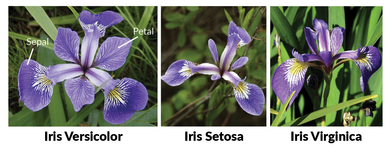
We introduced the iris data set in Section 2 - a native R data set that you can just access without needing to load anything.
It contains information on iris flowers of different species and we will use the glimpse() function from dplyr to get a first overview of the data we have at hand:
dplyr::glimpse(iris)
# Rows: 150
# Columns: 5
# $ Sepal.Length <dbl> 5.1, 4.9, 4.7, 4.6, 5.0, 5.4, 4.6, 5.0, 4.4, 4.9, 5.4, 4.…
# $ Sepal.Width  <dbl> 3.5, 3.0, 3.2, 3.1, 3.6, 3.9, 3.4, 3.4, 2.9, 3.1, 3.7, 3.…
# $ Petal.Length <dbl> 1.4, 1.4, 1.3, 1.5, 1.4, 1.7, 1.4, 1.5, 1.4, 1.5, 1.5, 1.…
# $ Petal.Width  <dbl> 0.2, 0.2, 0.2, 0.2, 0.2, 0.4, 0.3, 0.2, 0.2, 0.1, 0.2, 0.…
# $ Species      <fct> setosa, setosa, setosa, setosa, setosa, setosa, setosa, s…
Imagine...
When working with "real" data, aka survey or experimental data, we will usually need to reshape, filter and generally edit the data a bit. This may sound a bit sketchy at first, but we do not want to fake or change any data, we just want to ensure that we have the highest-quality data set to work with that we can.
In the example we will be working with, we have the following three goals for the data:
- We only want data from species "virginica".
- We are interested in sepal length.
- We want to adjust variable names.
- We later also want the species to be capitalized in our data & to add a new binary variable for whether a flower's petals are longer than 5.5 cm (1) or not (0).
Using dplyr functions, we can easily achieve all these goals in a few lines of code.
We will go more into depth
library(dplyr)

iris_virginica <- iris %>% # create new data set as copy
  filter(Species == "virginica") %>% # 1. only virginica
  select(Petal.Length, Species)  %>% # 2. select columns
  rename(plength = Petal.Length) # 3. rename variable/column

str(iris_virginica)
# 'data.frame': 50 obs. of  2 variables:
#  $ plength: num  6 5.1 5.9 5.6 5.8 6.6 4.5 6.3 5.8 6.1 ...
#  $ Species: Factor w/ 3 levels "setosa","versicolor",..: 3 3 3 3 3 3 3 3 3 3 ...
4.3.1 Filter
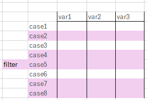
- Filters data by a value in a variable
- With filter we keep only certain rows in our data
- Needs logical operators as input
- "keep only cases where variable x has value abc"
- Can also be used with the ! to drop certain cases
- Drop NAs:
data %>% filter(!is.na(variable))
4.3.2 Select
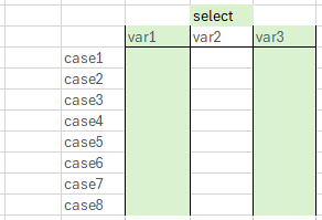
- Selects variables based on their names
- With select we keep only certain columns in our data
- Needs variable names as input
- "keep only variables with this name"
- Can also be used with the ! to drop certain variables
- Cave: if we want to extract one variable to calculate something, you will want to use
pull()instead- Check
iris %>% select(Species) %>% class()andiris %>% pull(Species) %>% class()
- Check
4.3.3 Rename
This is probably the most intuitively named function: It renames a variable in a data frame. As input the function takes your new variable name, an equal sign and the old variable name. This order is important, so if you run into an error, make sure that you are using new_variable = old_variable. Also, you do not need quotes around your variable names.
4.3.4 Mutate
- We also want the species to be capitalized in our data
- We also want to add a new binary variable for whether a flower's petals are longer than 5.5 cm (1) or not (0)
- for this, we use the
ifelse()function: - Needs a logical as first input, then what to do if it's true, last what to do if it's false
- for this, we use the
- Mutate takes a variable name as input (existing or new) and some function or calculation to be done on that variable
4.3.5 group_by & summarize
- With the dplyr-workflow, we can easily output group statistics
- Keywords: group_by() & summarize()
- The code is built like any other dplyr workflow with pipes ( %>% ) in between each:
- Define/ name the data frame
- group_by(variable_name)
- in summarize, define a name for the statistic, use a =, use a function like mean() for the measure
str(Orange) # use different default data set
# Classes 'nfnGroupedData', 'nfGroupedData', 'groupedData' and 'data.frame':    35 obs. of  3 variables:
#  $ Tree         : Ord.factor w/ 5 levels "3"<"1"<"5"<"2"<..: 2 2 2 2 2 2 2 4 4 4 ...
#  $ age          : num  118 484 664 1004 1231 ...
#  $ circumference: num  30 58 87 115 120 142 145 33 69 111 ...
#  - attr(*, "formula")=Class 'formula'  language circumference ~ age | Tree
#   .. ..- attr(*, ".Environment")=<environment: R_EmptyEnv>
#  - attr(*, "labels")=List of 2
#   ..$ x: chr "Time since December 31, 1968"
#   ..$ y: chr "Trunk circumference"
#  - attr(*, "units")=List of 2
#   ..$ x: chr "(days)"
#   ..$ y: chr "(mm)"

Orange %>%
  group_by(Tree) %>%
  summarize(m_age = mean(age),
            m_circumference = mean(circumference),
            n = n())
# # A tibble: 5 × 4
#   Tree  m_age m_circumference     n
#   <ord> <dbl>           <dbl> <int>
# 1 3      922.            94       7
# 2 1      922.            99.6     7
# 3 5      922.           111.      7
# 4 2      922.           135.      7
# 5 4      922.           139.      7
Exercises
Data Munging
Imagine we want to edit the iris data set for our colleagues from the US, who are interested in the petal width of the setosa and versicolor species.
- Create a new dataset from
iriswith a meaningful name select()the variables of interestfilter()the species that we want- Use %in% to filter by more than one value, or think about a reverse approach...!
rename()the Petal.Width variable to be named pwidth- Use
mutate()to add a new variable named "pwidth_inch", which contains the petal width in inches- Calculation: pwidth / 2.54 (2.54 cm = 1 inch)
iris_twospec <- iris %>%
  select(Petal.Width, Species) %>%
  filter(Species %in% c("setosa", "versicolor")) %>%
  # or: filter(Species != "virginica")
  # or: filter(Species == c("setosa" | "versicolor"))
  rename(pwidth = Petal.Width) %>%
  mutate(pwidth_inch = pwidth / 2.54)

head(iris_twospec, 8)
#   pwidth Species pwidth_inch
# 1    0.2  setosa  0.07874016
# 2    0.2  setosa  0.07874016
# 3    0.2  setosa  0.07874016
# 4    0.2  setosa  0.07874016
# 5    0.2  setosa  0.07874016
# 6    0.4  setosa  0.15748031
# 7    0.3  setosa  0.11811024
# 8    0.2  setosa  0.07874016
Group Statistics
Follow the structure to group the iris data set by Species and output a summary with the mean values of all four other variables in the data.
Also include the grouped n.
iris %>%
  group_by(Species) %>%
  summarize(m_plength = mean(Petal.Length),
            m_pwidth = mean(Petal.Width),
            m_slength = mean(Sepal.Length),
            m_swidth = mean(Sepal.Width),
            n = n())
# # A tibble: 3 × 6
#   Species    m_plength m_pwidth m_slength m_swidth     n
#   <fct>          <dbl>    <dbl>     <dbl>    <dbl> <int>
# 1 setosa          1.46    0.246      5.01     3.43    50
# 2 versicolor      4.26    1.33       5.94     2.77    50
# 3 virginica       5.55    2.03       6.59     2.97    50
Piping Hot %>%
You already heard about the pipe operator in Section ??.
The pipe - available as a native R pipe |> or a tidyverse pipe from the magrittr package %>%4 - takes the input from the left-hand to the right-hand.
In simpler terms, it takes the operation you did before the pipe and uses is as input for the function after the pipe.
This keeps our code readable and tidy and allows us to keep edits in separate lines, but we still only have to run one command for every task we need
It's easy to add new commands by using another pipe operator, or to leave edits out but commenting out the respective line of code.
It is important to say that most things can be achieved with or without pipe and you may prefer different versions for different tasks. You have seen a basic example of the use of the pipe operator in Section ??, so now we will look at a more sophisticated example: We will perform similar operations as we did above and code them first with pipe and then without.
# With pipe
iris_edit <- iris %>%
 filter(Petal.Length > 3) %>% # only big petals
 select(Species, Petal.Length, Sepal.Length) %>%  # only those columns
 mutate(random_calculation = Petal.Length * Sepal.Length) # calculate random new variable

# Without pipe - two versions
iris_edit2 <- filter(iris, Petal.Length > 3)
iris_edit2 <- select(iris_edit2, Species, Petal.Length, Sepal.Length)
iris_edit2 <- mutate(iris_edit2, random_calculation = Petal.Length * Sepal.Length)

iris_edit3 <- mutate(
  select(
    filter(
      iris, Petal.Length > 3
    ),
    Species, Petal.Length, Sepal.Length
  ),
  random_calculation = Petal.Length * Sepal.Length
)

# Are the three versions equal?
all.equal(iris_edit, iris_edit2) & all.equal(iris_edit, iris_edit3)
# [1] TRUE
As you can see, all three version produce the same output and all are technically correct. However, in the second example we keep re-assigning new edits to the same data frame (would be even more annoying but possible to assign each edit to a new data frame) and the third version is just quite the nightmare to read if you ask me. Also think about this:
In the part with pipe we used the
irisdata to edit and assigned it toiris_edit. In version two without pipe we usedirisin the first line, but afterwards we usediris_edit2for assignments and edits.
Why is that?
If we were to use iris in each line, it would overwrite the last edit every time.
We can also profit from the pipe in base-R or with a larger combination of different functions. Usually, the pipe helps us not to drown in parentheses when conducting analyses. Let's e.g. calculate a mean value after filtering by Species setosa.
So without a pipe, it might look like this:
Using all pipes, the code would look a lot longer but still easier to read.
iris %>%
filter(Species == "setosa") %>%
pull(Petal.Length) %>%
mean() %>% round(digits = 2)
# [1] 1.46
As a third alternative, we might also use a combination of the approaches, such as:
As with most things in R and programming, different approaches may be easier in different situations, so it has merit to think outside the box at times!
Brainteaser : We want to edit the iris data to rename a Petal.Length to pl and mutate it to be multiplied by ten. Why does the first version work, but not the second one?
# Version 1
iris %>%
  mutate(Petal.Length = Petal.Length * 10) %>%
  rename(pl = Petal.Length) %>%
  glimpse()

# Version 2
iris %>%
  rename(pl = Petal.Length) %>%
  mutate(Petal.Length = Petal.Length * 10) %>%
  glimpse()
In the second version, we rename the variable Petal.Length to pl and afterwards try to access it with its old name.
Wrap-Up & Further Resources
- Packages make working with R easier
-
dplyris a powerful tool for editing data (select, filter, mutate...) - The pipe %>% makes your code clearer and "follows the thought process"
- R for Data Science Book
- dplyr vignette
- Pipe operator
- Cheatsheet: https://github.com/rstudio/cheatsheets/blob/main/data-transformation.pdf
- YouTube: 20 R Packages that you should know - you for sure don't need them all, but there are some nice inspirations for working with packages in there

Being able to read your own code after a while is already challenging but try making sense of code that someone else has written!↩︎
The two pipes can pretty much the same operations - for specific differences see https://www.tidyverse.org/blog/2023/04/base-vs-magrittr-pipe/↩︎